1.5 ImageJ Module

Overview

The ImageJ module allows users to execute arbitrary ImageJ macros on single images or datasets of images. Macro parameters can be changed and parameter value lists can be provided to experiment with parameter variations. The results are stored back in BisQue as Gobjects, tables, or images.

---

Uploading of ImageJ Pipelines

Most ImageJ macros can be uploaded and used directly with minor modifications. In order to upload a macro, click “Upload”, select the macro file, and click “Upload”. If the file extension is “.ijm”, the file will automatically be recognized as a CellProfiler macro.

As an example, we upload the CometAssay macro developed at the Microscopy Services Laboratory of the University of North Carolina at Chapel Hill, Comet Assay.

In order to verify the macro, it can be opened by browsing the imagej_pipeline resources and opening the recently uploaded macro.

It will look like this:

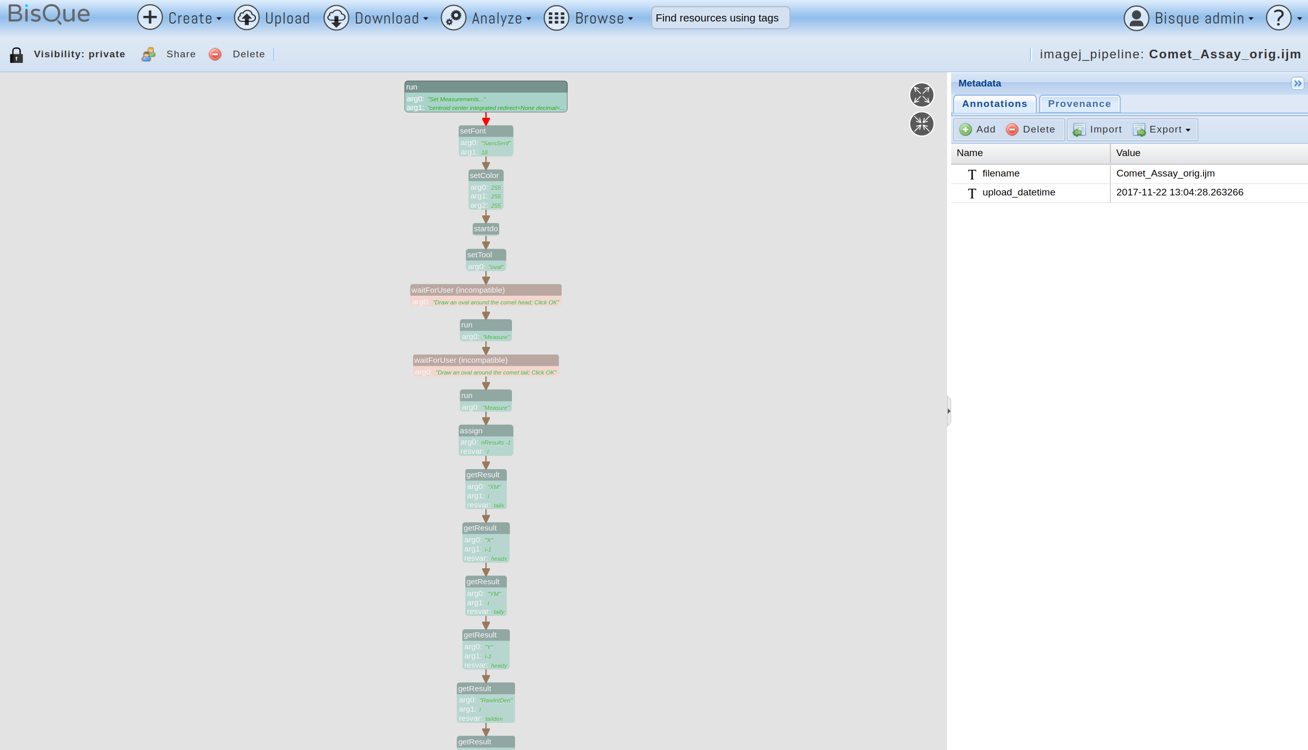
ImageJ Pipeline

Each box represents one ImageJ macro step and the arrows indicate the flow through the steps. Note that some boxes have different colors. For example, the “waitForUser” and “Dialog”-related boxes are shown in red to indicate that they are incompatible with BisQue and will render the macro non-executable. Green boxes indicate regular ImageJ steps that were kept unchanged. Blue boxes are BisQue specific steps (such as “load image from BisQue” or “store table to BisQue”).

In order to execute the pipeline, we need to fix the red boxes and then re-upload the pipeline. In this example, the first red boxes correspond to the waitForUser steps of the macro:

waitForUser("Draw an oval around the comet head; Click OK");
run("Measure");
waitForUser("Draw an oval around the comet tail; Click OK");
run("Measure");

Since BisQue modules are currently not interactive, such steps are not allowed. However, since they request user-defined regions for head and tail of the comet to analyze, we can replace them with BisQueLoadPolygon steps:

BisQueLoadPolygon("head");
run("Measure");
BisQueLoadPolygon("tail");
run("Measure");

Each BisQueLoadPolygon step searches for a polygon Gobject in the current image and returns it as an ImageJ selection.

The other red boxes correspond to ImageJ “Dialog” functions:

Dialog.create("Do Another?");
Dialog.addCheckbox("Yes", true);
Dialog.show();

Again, since BisQue is not interactive, these are not allowed. In this example, these steps check if the user wants to analyze more comets. For simplicity, we will simply remove these steps and end the analysis after one iteration.

This addresses all red boxes but before being able to run the macro in BisQue, we need to add two important steps: the input and output. For the input, we can just add a new step at the very beginning:

BisQueLoadImage();

This will load the current image of the module execution into ImageJ for analysis. Note that for larger datasets of images, the macro will be executed once for each image.

For the output, we will store the comet analysis results as a table back into BisQue. This is achieved by adding the following line at the end of the macro:

BisQueSaveResults("comet stats");

This step will read the ImageJ results table and store it in BisQue under the given name. It will be linked in the output section of the current MEX (module execution) document.

The completed macro is now as follows:

BisQueLoadImage();
run("Set Measurements...", "centroid center integrated redirect=None decimal=3");
setFont("SansSerif", 18);
setColor(255, 255, 255);
BisQueLoadPolygon("head");
run("Measure");
BisQueLoadPolygon("tail");
run("Measure");
i = nResults -1;
tailx = getResult("XM", i);
headx = getResult("X", i-1);
taily = getResult("YM", i);
heady = getResult("Y", i-1);
tailden = getResult("RawIntDen",i);
headden = getResult("RawIntDen",i-1);
CometLen = sqrt( ((tailx-headx)* (tailx-headx)) + ((taily-heady)*(taily-heady)) );
setResult("TailLen",i,(CometLen));
setResult("TailMoment",i , (CometLen * tailden));
setResult("%TailDNA",i ,(tailden/(tailden + headden))*100);
updateResults();
BisQueSaveResults("comet stats");

After uploading this macro again, all boxes are either green or blue, indicating the pipeline is now valid for execution.

---

Running an ImageJ Macro

ImageJ macros can be run like any other BisQue module. First, select the macro to run (in this example, we select the CometAssay macro. After viewing the pipeline, click on “Analyze” and then on “ImageJ”. The ImageJ module page opens. Click “Select an Image” to choose a single image to run the macro on (alternatively, a dataset of images can be selected to run the macro on multiple images in parallel):

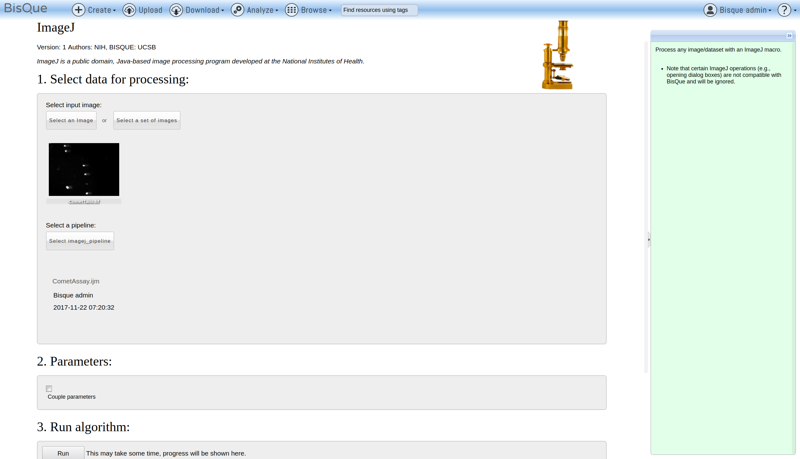
ImageJ Pipeline

Note that the selected image(s) need to have at least two polygon Gobjects: one with semantic type “head” and one with semantic type “tail”.

Finally, click the “Run” button to start the macro execution.

Once the execution finishes, the outputs are shown in section 4:

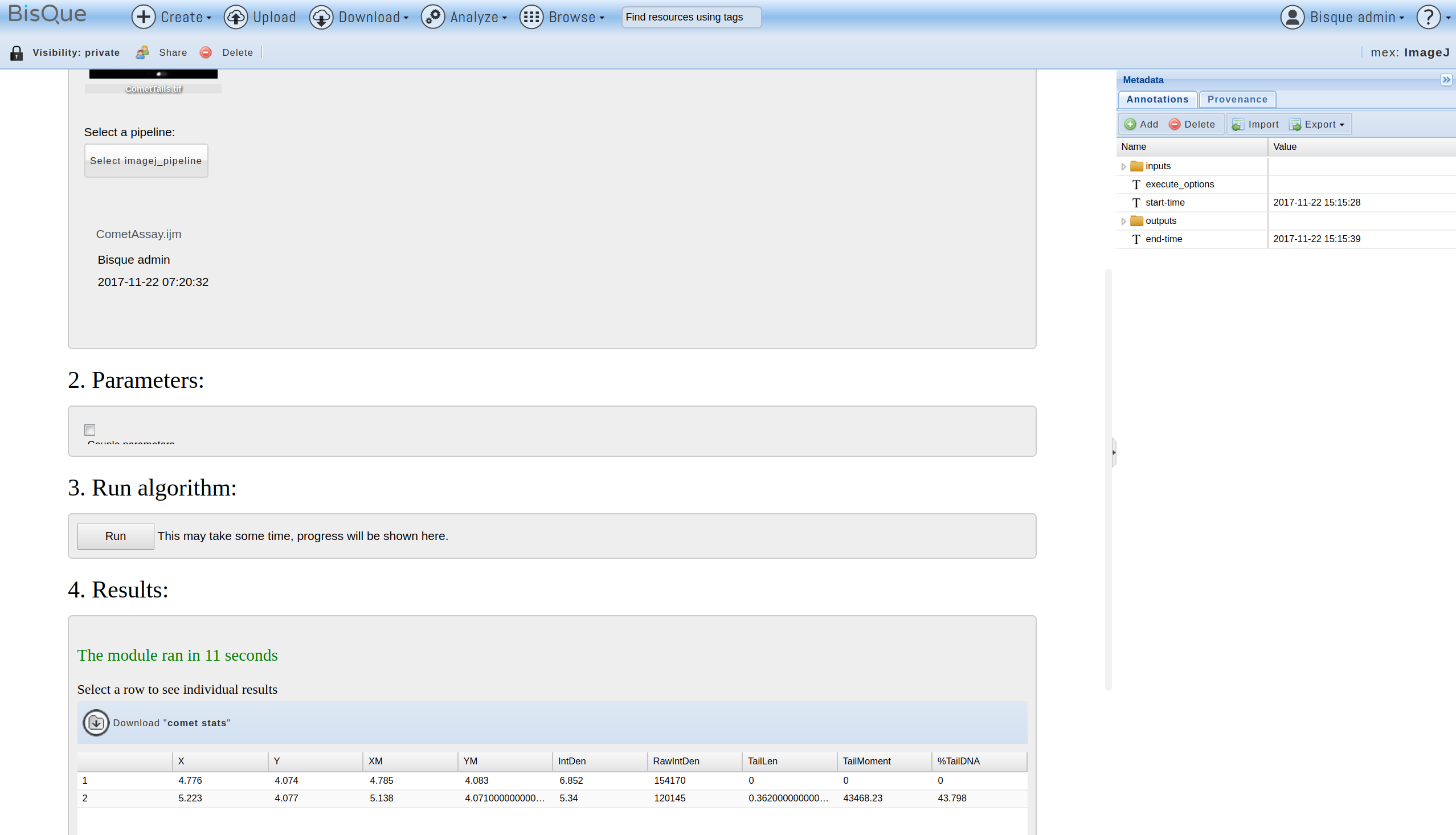
ImageJ Pipeline

In this case, one table “comet stats” was generated. It contains the comet statistics computed in the macro. Depending on the macro, images or Gobjects can also be generated as output (see next section).

The generated tables can now be processed further in additional BisQue modules or shared with other users.

---

Special BisQue extensions for ImageJ

There are several BisQue-specific extensions to ImageJ to allow ImageJ macros to interact with the BisQue system. Each one is described in the following.

BisQueLoadImage()

This function corresponds to the open() function of ImageJ. Instead of opening an image from a file, however, it obtains the image from the BisQue module executor. The opened image is one of the images from the module input section.

BisQueLoadPolygon("gobject type")

This function loads a polygon Gobject from the current image into ImageJ as a selection for further processing in the macro. The “gobject type” parameter is used to select a specific Gobject with the semantic type “gobject type”. In other words, the current image has to have a Gobject as follows:

<gobject type="gobject type">
  <polygon>
    <vertex index="0" t="0.0" x="735.0" y="617.0" z="0.0"/>
    ...
    <vertex index="10" t="0.0" x="727.0" y="624.0" z="0.0"/>
  </polygon>
</gobject>

This can be generated for example via the graphical annotations tool in the BisQue image viewer.

BisQueSaveImage("image name")

This function corresponds to the saveAs("Tiff", ...) function of ImageJ. Instead of saving the image to a file, however, it stores the image back into BisQue as a new image resource. The created image is then referenced in the MEX (module execution) document’s output section.

BisQueSaveROIs("polygon", "label", "color")

This function stores the current ImageJ ROIs as polygon Gobjects in the output section of the current MEX (module execution) document. Each polygon is assigned the provided label and color.

BisQueAddTag("tag_name", "tag_value")

This function adds a tag/value pair to the output section of the current MEX (module execution) document.

BisQueSaveResults()

This function stores the current ImageJ result table as a table resource in BisQue. The created table is then referenced in the MEX (module execution) document’s output section.